Renew Your Office Workflow with AI Companion: Let's Collaborate Claude, Excel, and Word

Overview

AI usage enable us to have a fast productivity boost. By using AI, we can renew our Office workflow using the help of AI Companion. Claude is the main AI model/platform will be used in this session.

Claude, especially Claude Desktop has the ability to connect to MCP servers. This allows Claude to access our Excel file without the need to upload it manually. This also allow us to connect to various MCP servers.

Let's make this session a safe place to learn. Don't hesitate to ask questions. If you have completed several steps, please feel free to assist other participants who might need help.

Prerequisites

Internet connection
Microsoft Office 2016 or above, or Microsoft Office 365
Claude Desktop installed
Claude account
Bun and uv installed to start MCP server
Stay calm and enthusiastic!🔥

Bun Installation

Follow instructions below based on your operating system.

macOS

Open Terminal

Run the following command:

curl -fsSL https://bun.sh/install | bash

Close and reopen Terminal
Type bun --version to verify that Bun was installed successfully

Windows

Open Terminal or PowerShell

Run the following command:

powershell -c "irm bun.sh/install.ps1 | iex"

Close and reopen Terminal or PowerShell
Type bun --version to verify that Bun was installed successfully

uv Installation

Follow instructions below based on your operating system.

macOS

Open Terminal

Run the following command:

curl -LsSf https://astral.sh/uv/install.sh | sh

Close and reopen Terminal
Type uv --version to verify that Bun was installed successfully

Windows

Open Terminal or PowerShell

Run the following command:

powershell -ExecutionPolicy ByPass -c "irm https://astral.sh/uv/install.ps1 | iex"

Close and reopen Terminal or PowerShell
Type uv --version to verify that Bun was installed successfully

Create a Working Directory

Go to Finder or File Explorer, then create a folder. This folder will be your main working folder for this session.
Copy your path to the folder and store in a text editor to be used for the next step.

Connect MCP Servers to Claude Desktop

Open Claue Desktop
Click on the profile icon on the bottom left
Select "Settings"
Go to "Developer" tab
Click on "Edit Config" button
Open the claude_desktop_config.json file on the text editor (Notepad, TextEdit, or VS Code)

Insert the following code at the beginning of the JSON file:

{
  "mcpServers": {
    "filesystem": {
      "command": "bunx",
      "args": [
        "-y",
        "@modelcontextprotocol/server-filesystem",
        "<your_working_directory_path>"
      ]
    },
    "markitdown": {
      "command": "uvx",
      "args": ["markitdown-mcp"]
    }
  },
  "... other existing settings ..."
}

Save the file and close the text editor
Restart Claude Desktop for the changes to take effect
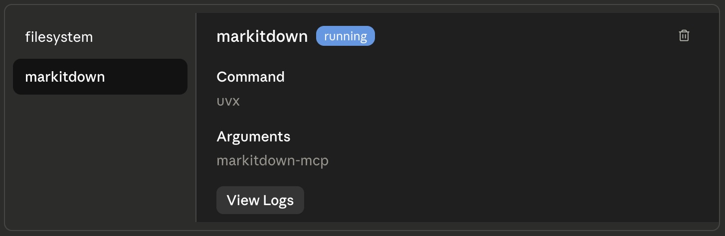
Repeat step 1 to 4, make sure the filesystem and markitdown MCP connection running.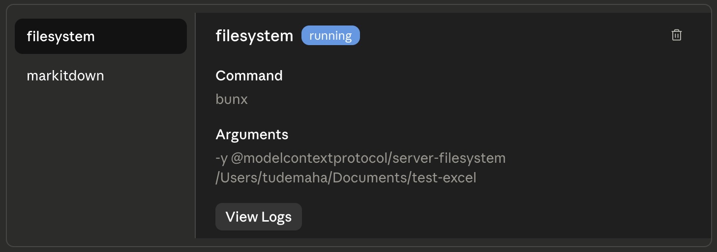

In this section, we will create a dynamic schedule table for an event rundown. By using this table, we only need to know the event's start time and duration for each activity. The table will automatically calculate the end time for each activity.

If you want, download this Excel file then move it to your working directory to make it easier to follow.

Create an Excel file, let's name it rundown.xlsx, and save it in your working directory.
Create a table with this headers: "No", "Time", "Duration", and "Activity" following the example below.
At cell B2, enter the starting time of the event, for example 08:00.
At cell D2, enter a formula =B2+TIME(0;E2;0) where E2 is the duration of the activity in minutes.
Enter the duration of the first activity in minutes at cell E2, for example 30. Cell D2 will automatically show the end time of the activity.
At cell B3, enter a formula =D2, it will be the starting time for the second activity.
At cell D3, we will use the same formula as on step 4, but on different cell reference, so it will be =B3+TIME(0;E3;0).
Enter the duration of the second activity in minutes at cell E3, for example 45.
Repeat step 6 to 8 to fill in the rest of the table with adjustment of the reference cell, or you can block range B3:D3, drag the fill handle to the bottom right of the last cell in the range, then release the mouse button. The formula will automatically adjust the reference cell.
Now you have a dynamic rundown table, you can change the start time or duration of any activity and the table will automatically update.
Use the "Format Painter" tool to copy the format of the first row to the rest of the rows.

After finishing the steps, you will have this dynamic rundown table. Finished Rundown Table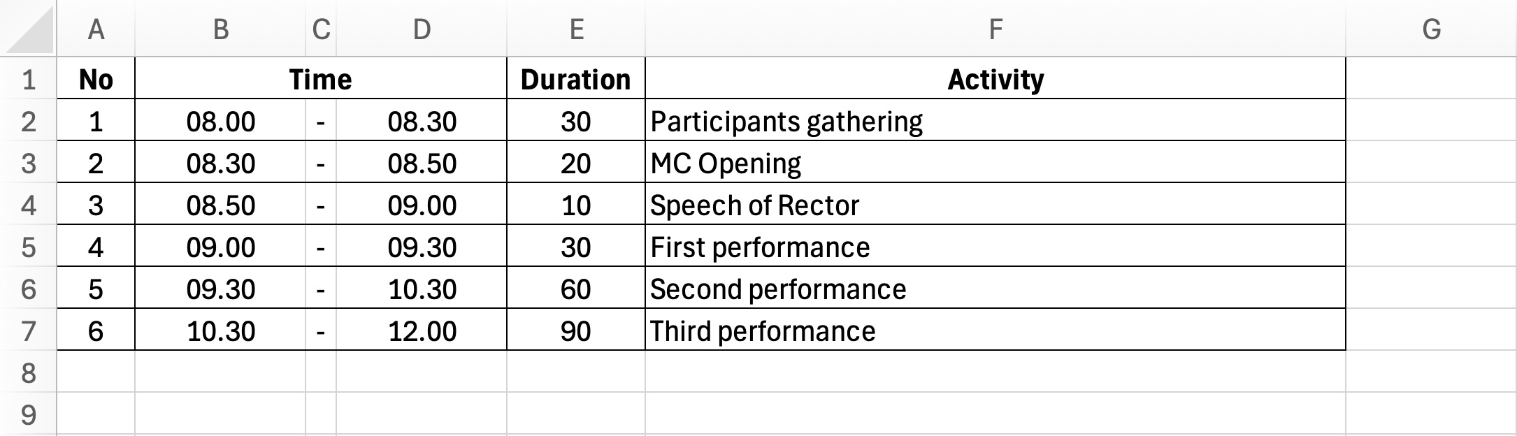

Download this Excel file then move it to your working directory.

Open Claude Desktop

Try to ask this question

Read "dataset-penjualan.xlsx" using `filesystem` MCP tool, then use `markitdown` MCP tool to convert the file into markdown for efficien reading, if needed. Then, tell me, what is the dataset about?

Baca "dataset-penjualan.xlsx" pakai MCP `filesystem`, terus pakai MCP `markitdown` but konversi file itu jadi markdown biar bacanya lebih efisien, kalau perlu. Terus, kasi tau aku, tentang apa dataset itu?

Click "Allow once" or "Always allow" if needed.
Claude will read the file and convert it into markdown, then tell you what the dataset is about.
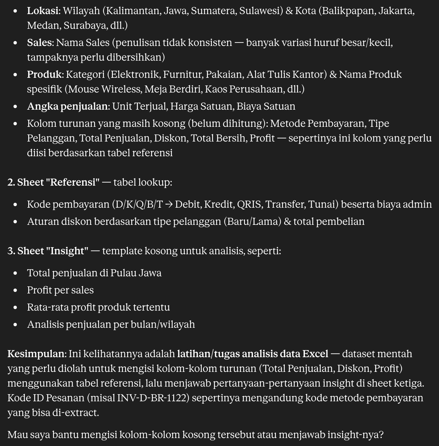
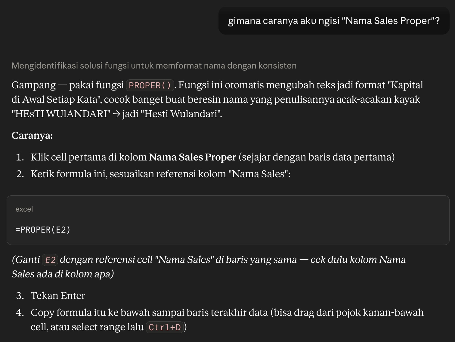
Now, try to ask on how to fill the "Nama Sales Proper" to Claude. It will give you the answer.

At cell K2, enter a formula =PROPER(E2) where E2 is the "broken" name format, as Claude said.
Metode Pembayaran column should be filled with the payment method from the reference table. The fifth letter of the ID Pesanan is the payment code. Use this formula referenceto fill cell L2:
```
=VLOOKUP(MID(A2;5;1);Referensi!$A$1:$C$6;2;FALSE)
```
Tipe Pelanggan column should be filled with Lama or Baru based on the seventh and eighth letters of the ID Pesanan. BR is Baru and LM is Lama. Use this formula reference to fill cell M2:
```
=IF(MID(A2;7;2)="BR";"Baru";"Lama")
```
Total Penjualan is a multiplication of Unit Terjual and Harga Satuan column. Use this formula reference to fill cell N2:
```
=I2*H2
```
Column Diskon (%) must be filled in carefully. Look at the reference table, there is the rule to give discount for each purchase. Understand the reference table or ask Claude on how to fill this column. Formula reference to fill cell O2:
```
=IF(AND(M2="BARU";N2>50000000);20%;IF(AND(M2="LAMA";N2>50000000);15%;IF(AND(M2="BARU";N2>20000000);10%;0%)))
```
Harga Setelah Diskon is Total Penjualan minus discount amount. Formula reference to fill cell P2:
```
=N2-O2*N2
```
Total Bersih is Harga Setelah Diskon minus the admin fee. The fifth letter of the ID Pesanan is the payment code. Use VLOOKUP to the reference table to get the admin fee. Formula reference to fill cell Q2:
```
=P2-VLOOKUP(MID(A2;5;1);Referensi!$A$1:$C$6;3;FALSE)
```
Profit is obtained by subtracting the Total Bersih from the Biaya Satuan tiap Unit Terjual. Formula reference to fill cell R2:
```
=Q2-(H2*J2)
```
To fill all the rows, block range K2:R2, drag the fill handle to the bottom right of the last cell in the range, then release the mouse button. The formula will automatically adjust the reference cell.
Total row is the sum of Total Bersih and Profit. Formula reference to fill Q222 and R222:
```
=SUM(Q2:Q221)
=SUM(R2:R221)
```
Rata-rata row is the averate of Total Bersih and Profit. Formula reference to fill Q223 and R223:
```
=AVERAGE(Q2:Q221)
=AVERAGE(R2:R221)
```
Use MAX function to get the maximum of Total Bersih and Profit. Formula reference to fill Q224 and R224:
```
=MAX(Q2:Q221)
=MAX(R2:R221)
```
Use MIN function to get the minimum of Total Bersih and Profit. Formula reference to fill Q225 and R225:
```
=MIN(Q2:Q221)
=MIN(R2:R221)
```

```

Jump to "Insight" sheet. We will answer the questions based on our finished dataset.

To get the total sales in Java, we can use SUMIF function on Total Bersih column based on the Wilayah column. Formula reference to fill cell B1:
```
=SUMIF('Data Penjualan'!C2:C221;"JAWA";'Data Penjualan'!N2:N221)
```
To count the sales in Kalimantan, we can use COUNTIF function on Wilayah column. Formula reference to fill the cell B2:
```
=COUNTIF('Data Penjualan'!$C$2:$C$221;"KALIMANTAN")
```
To know the sales profit at Surabaya, we need to sum all the profit in Surabaya city. Use SUMIF for this purpose. Formula reference to fill the cell B3:
```
=SUMIF('Data Penjualan'!$D$2:$D$221;"SURABAYA";'Data Penjualan'!$R$2:$R$221)
```
We need to add up all the USB-C Hub units sold to get the number of units sold. Use SUMIF function for this purpose. Formula reference to fill the cell B4:
```
=SUMIF('Data Penjualan'!$G$2:$G$221;"USB-C HUB";'Data Penjualan'!$H$2:$H$221)
```
To get the average profit of HD Webcam sales, use AVERAGEIF function on Profit column based on the Nama Produk column. Formula reference to fill the cell B5:
```
=AVERAGEIF('Data Penjualan'!$G$2:$G$221;"WEBCAM HD";'Data Penjualan'!$R$2:$R$221)
```

To find out the number of sales at Sulawesi in February, use COUNTIFS function on Wilayah and Tanggal Pesanan columns. Formula reference to fill cell B6:

=COUNTIFS('Data Penjualan'!$C$2:$C$221;"SULAWESI";'Data Penjualan'!$B$2:$B$221;">="&DATE(2024;2;1);'Data Penjualan'!$B$2:$B$221;"<="&DATE(2024;2;29))

Use SUMPRODUCT function to get the total sales in April. SUMPRODUCT function multiply corresponding rows of arrays and sum the result. Formula reference to fill cell B7:
```
=SUMPRODUCT('Data Penjualan'!$N$2:$N$221;(MONTH('Data Penjualan'!B2:B221)=4)*1)
```
To find the name of all sales, we can use UNIQUE function to get the unique values of Nama Sales Proper column. Formula reference to fill cell G3:
```
=UNIQUE('Data Penjualan'!K2:K221)
```
Lastly, to find profits generated by each sales, use the SUMIF function of the Profit column and each name. Formula reference to fill cell H3 and after:
```
=SUMIF('Data Penjualan'!$K$2:$K$221;Insight!G3;'Data Penjualan'!$R$2:$R$221)
```

To get a better insight, we can use PivotTable. We will create a PivotTable to show the profit of all products per category in each city. We will also add filter region and sale date.

Go to Data Penjualan sheet
Block the range A1:R221
Go to "Insert" > "PivotTable"
Make sure to select "New worksheet", then click "OK"
Rename the new sheet into "Pivot"
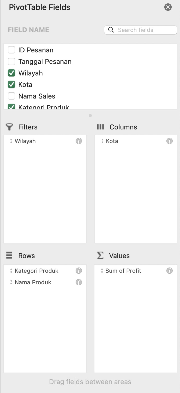
Drag and drop each field on the right panel to Filters, Columns, Rows, and Values section. Refer to the image below to get the layout:
Select the PivotTable created, go to "PivotTable Analyze" > "Insert Timeline"
Select Tanggal Pesanan, then click "OK"
You should now have a PivotTable like this:
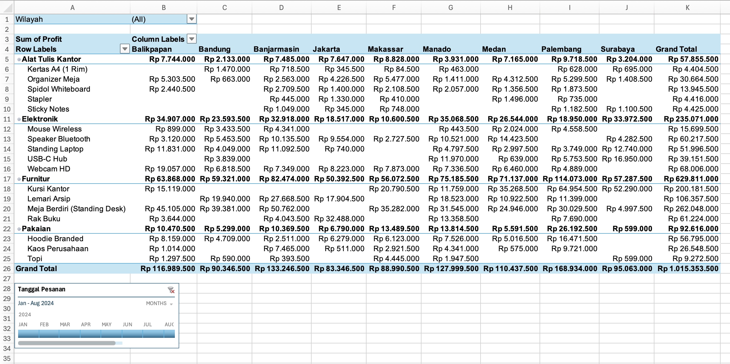
Now it's much easier to gain insights using PivotTables.

Ask Claude to Help You Generate the Report

After completing all stages, it's time to generate the report. Here's what Claude can do to help you:

I've filled the dataset, answer the questions, and generate a PivotTable. Now, I need to create a report based on that data. What should I put on the Word document to generate a insightful report?

Aku udah lengkapin datasetnya, jawabin pertanyaan di insight, dan buat PivotTable. Sekarang, aku perlu buat laporan berdasarkan data tersebut. Apa yang harus aku masukin ke dokumen Word biar laporanku informatif?

Additional Tips

Create different variations of PivotTable to make it easier for Claude to analyze the data. Here is some examples of the PivotTable:
Variation 1: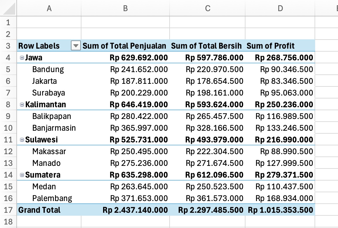

Variation 2: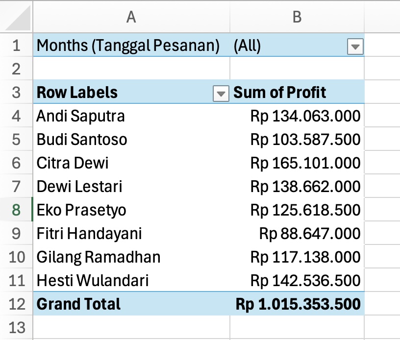
Pay close attention to what Claude generates. Make sure all of the data is correct. If it's incorrect, you can ask Claude to revise the report based on the data.
Edit the report generated by Claude. It will "humanize" the report, it will not look like generated by AI.
Add supporting charts and tables.

Author, Tude Maha, generate this Codelabs guide with the assistance of AI. These are the AI used:

Claude
- Generate dummy sales data, with modification
- Brainstorming assistance to create a simple-to-explain Excel functions
- Generate example of Claude usage for Excel and Word
- This AI is used because it is the main AI platform used for this workshop
Gemini
- Generate "broken" format for sales' name
- This AI is used to separate the main conversation with Claude and utilize its temporary mode